Migrating the “Unusual” into ArcGIS/ArcFM

At the conclusion of the movie Casablanca Captain Renault famously turns away from Rick and orders his sergeant to “round up the usual suspects.” (I love that movie – and I really love that line.) If we’re talking about migration of data into a utility or telco ArcGIS/ArcFM Geodatabase then the “usual suspects” include AutoCAD, Microstation, Smallworld and Intergraph. These products constitute the majority 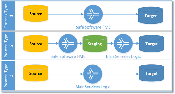from which customers migrate data into Arc. For these technologies we typically rely on Safe Software’s FME for some aspect of the migration process – either for extraction to a ‘staging’ database or for support of the entire migration pipeline.

There are, however, still products and home-grown GIS and mapping solutions that fall outside the boundary of the usual suspects. There are not FME Readers for these (we’re in the territory of “Process Type 3” in the diagram above.) In some cases there is not even documentation. So it may be the case that some level of “GIS Archeology” is required to uncover data structures and relationships essential to mapping a source system to a target ArcGIS/ArcFM data model.

Over the years we’ve had the opportunity to work with a number (*) of the “unusual suspects” and are pretty pleased to say have completed successful migrations from those sources into ArcGIS/ArcFM Geodatabases. We can also say that, though these systems might not be the most popular they are not necessarily poorly designed or implemented. Many factors contribute to success in the GIS marketplace, and technical excellence is only one of them – still we have had some “what were they thinking” moments along the way.

Thankfully there is always some level of commonality between any such system that makes the mapping and data migration possible in the first place. Among the important common properties are:

• All have some mechanism for distinguishing types of equipment, and for associating specific sets of attributes with those types.
• All have some way to describe geometries for spatial features, though the techniques vary widely.
• Most have some mechanism for describing what is connected to what – but again, mileage varies.

That said, here are some characteristics / categorizations we can apply to our “unusual suspects”:

• Asset systems that tag on an X, Y. If there is any level of commonality among these uncommon systems one is that the “mapping” component came about as somewhat of an afterthought to another, primary goal of the system. Almost as if someone building an asset management system in the middle of development had a “mapping” requirement thrust on them so they added X, Y fields onto a table and called it good.

In this case the core product itself may not actually render features in a map display, but rather provide the ability to extract data from the system in the form of an AutoCAD drawing or DXF file and provide some ability to mine the drawing afterward for updates that need to be applied to the asset database. In this case it can be tempting to use the AutoCAD drawing(s) as the source for migration – but this would be wrong and result in an incomplete migration process. The DWG/DWF is essentially a “report” representing a partial view of the data. A complete migration needs to go to the true data source.

A related characteristic is that coordinates are stored in a single, presumed coordinate system. There is no “spatial reference” property as we would find in an ArcGIS geometry definition that allow the geometry to be projected. So… we need to learn the presumed projection (typically a state plane or UTM grid) from some other source.

• Adding “shape” points. Of course even those systems with limited goals for “mapping” realize that adding an X, Y alone won’t meet basic mapping requirements. Some equipment is linear. And there might even be an occasional 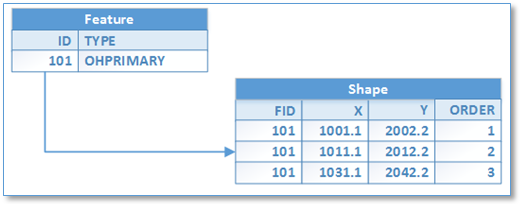requirement to represent a polygon. We’ve seen interesting ways to accomplish this, the most straightforward of which is to add a table with “shape” points, as illustrated here. From a migration standpoint, the presence of a “shape” table is a welcome sight. It means we can likely reproduce the original cartography with high fidelity.

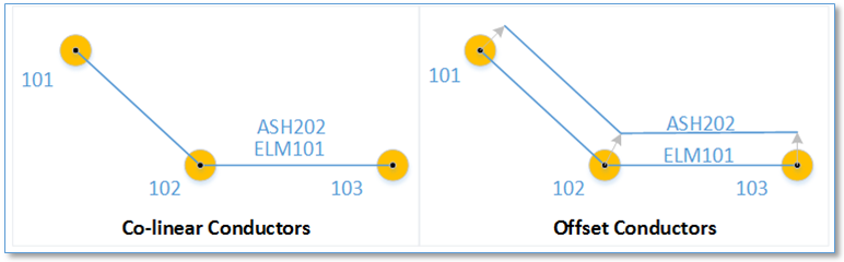
In other cases the shape of a linear feature may need to be inferred based on what the equipment is connected to or what its supported by. In the example illustrated below we would need to obtain 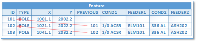the location of an electric conductor using the location of its “from” and “to” poles (or from and to structures to be inclusive of underground equipment). Seems simple at one level, but complexities are raised when there are multiple conductors on a pole line, especially when our target is an ArcGIS geometric network that relies on geographic coincidence to establish connectivity. With special processing that includes offsetting logic we would end up with coincident features that result in a bunch of unwanted “loops.” While some manual clean-up was required on completion of the automated process, the diagram below illustrates a portion of a strategy we employed to account for this condition.

• Connectivity table. It may be that in addition to the comparatively simple task of plotting X, Y coordinates the system seeks to maintain a representation of network connectivity, though the connectivity may be relatively coarse and may not correspond to how we would expect connectivity to be presented in an ArcGIS geometric network. An example for an electric distribution network is a simple device hierarchy table that contains each device and its parent. Such “device-parent” tables have been critical components of historical asset management systems and can help a company quickly answer questions such as “what customers are served under what device.” However another aspect of device-parent tables is that they are quite difficult to maintain and thus prone to error. Good thing GIS technology has matured to the point of being able to table over this responsibility!

The table may, or may not distinguish between a “parent” device which is simply a device immediately upstream of the current device from 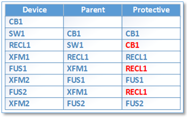a “protective parent” device which is the next upstream device that has the ability to open when excessive current from a downstream fault is induced. Knowing the parent protective device could be important for supporting applications such as outage management. Adding the protective parent column would result in a table as that at the right.

The connectivity table may be much more complex and may include associations among all network equipment, even to the point of describing associations between current-carrying equipment and the structures that support that equipment and attachments to support structures. An illustration is to the right. In this case the “topology” table includes definitions of not only what is connected to what, but also the manner in which they are connected. Mining a topology table 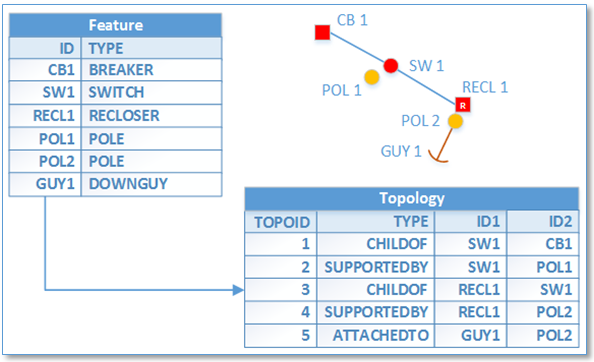such as this in a data migration context can provide the ability to help ensure that ArcGIS network connectivity is correct but also can help building relationships – such as the “Structure Relate” relationship often present in ArcFM utility Geodatabases.

A further variation on this theme is the case where a network is comprised of links, and nodes and points – with links connected to one another at nodes and that have points also potentially connected to nodes. In some cases there may be more than one point feature connected to a node. So envision the case of a gas distribution network where three pipes meet at a node and that two point features, a tee and a reducer are also connected to the node.

Whatever manner of connectivity may be defined explicitly in the source database it can only help so much in establishing comparable connectivity in the target ArcGIS geometric network, with the key reason being that the geometric network relies on 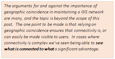geographic coincidence and in systems with connectivity tables the feature geographic location is (or at least can be) completely independent of network connectivity.

So, what does this all mean for our data migration task? Well, a variety of things depending on the exact content of the source database. But it might mean that we can only use the connectivity table as a means to validate results and not as a tool that can be used directly in the migration process. Consider the following example.

In this case we may have discovered feature geometries from a “shape” table and have device connectivity in a separate “parent device” table, but the two are not related. The best we might be able to do is determine cases where a device parent in our target ArcGIS/ArcFM Geodatabase differs from the device parent as defined in the source database.

A convenient way to do this is to take advantage of the ArcFM Objects method IMMElectricTracingEx.TraceDownstream. This returns a set of junction network elements downstream of a starting point, typically a feeder circuit breaker. Importantly, the method also returns the parent junction for each network junction traced, allowing us to walk upstream from any device and identify its parent – or with a little extract logic determine its protective parent.

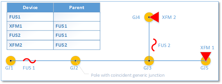
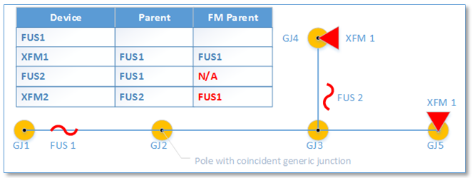
Below is a depiction of what our trace results might show from the example above. Specifically we would see that transformer XFM1 has a different parent and FUS2 has no parent. In this simple example the cause is quite clearly the fact that FUS2 is offset from the primary line and not included in the network (of course we could have also seen this issue by inspecting our geometric network build errors.) However, a point to keep in mind through this process is that the discrepancy we see between source and target network representations could be due to an error in the source network.

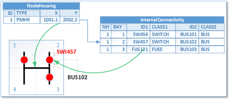
• Internal Connectivity. In some specialized cases a source system may have particular rules and data structures for associating equipment in enclosures such as fiber optic cable patch locations or electrical distribution system switch cabinets. In such cases there may only be a geometry definition for the enclosure location itself and the remaining geometries and relationships must be generated from an associated internal connectivity table. Below is an example illustrating a migration strategy we employed in a similar case.

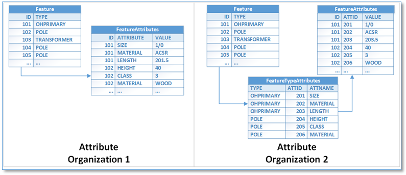
• Attribution. Feature attributes may be stored in discrete tables per equipment type – similar to the ArcGIS model – or there may be a single table containing attributes for all features organized as key-value pairs as illustrated to the left below. A variation on this approach is that there may be a look-up table defining attribute types associated with a feature that is required to join a particular feature definition to its attributes. In either case a compelling aspect of this organization is that no data model changes are required to add or alter attributes associated with an equipment type. Though that’s academic. Either source model can be accommodated in the data migration process.

Conclusion
We’ve offered a brief survey of some common characteristics of GIS/mapping system that we’ve found to fall outside the mainstream of current use and some of the migration strategies we’ve employed to successfully move this data into ArcGIS/ArcFM Geodatabases. Though there is some effort in constructing and configuring the logic for specialized processing, the fact that the whole (or vast majority) of the process can be automated and is repeatable can provide significant benefits given that migrations of this type typically need multiple iterations to perfect.